Scaling Sample Processing

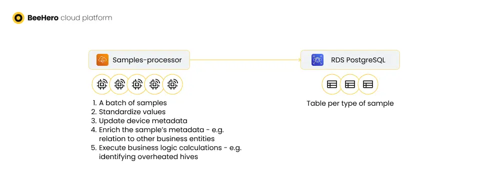
Sample processing is the phase in our IoT flow that transforms raw data into actionable data and business logic. It has several responsibilities:

• Translate firmware-specific sensor values into standardised values, and maintain the information about the IoT devices (e.g their firmware version)
• Enrich the sample with business data - for example, associating it with the beekeeper account the sample ‘belongs’ to, and associating it with a real-world physical entity (such as an orchard) where the hive is placed
• Execute additional business logic - identifying IoT conditions (for example, gateways being moved from storage to orchard), updating the orchard with the number of deployed hives and more

‍
With the scale of samples continuously growing, the processing phase posed several challenges:

• It was initially implemented as an HTTP server, which handled batches of samples in each request. We covered in our previous post the downsides of the HTTP server approach and how we transitioned to SQS beanstalks. The sample batches also became more of an issue, as a batch could include data from various devices, complicating DB queries and their result processing - the code had to first collate devices for the query and then separate the results during processing by device
• The implementation was ‘heavy’ on DB queries, both reading and updating information, which led to table locking while one request was updating the devices information and another was trying to read the same tables - exacerbated by the batch processing as parallel processes handled similar subsets of devices
• The process was more brittle due to many logic-intensive calculations. Unexpected code flows while handling a sample could delay or even fault an entire batch and complicate retry attempts - separating what was processed in the batch from what was not

‍

From batch processing to single sample processing

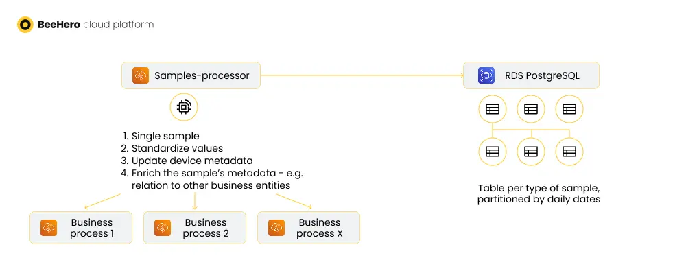
Batch processing is actually often a tool to increase scalability, but in this case it introduced the issues instead of solving them. Possibly if we could group the samples by device before processing (and guarantee that batches of the same device are not handled in parallel) it would work out, but at the time this was far from trivial. Instead, we opt to simplify the processing by running it for each sample separately, with a guarantee on the order of samples. Single sample processing resulted in each process only ever ‘touching’ one device, which greatly reduced table locking and the potential for race conditions between processors.
Order was guaranteed by the raw processor, the phase before the sample processing, which still worked in batches and was able to order those batches and send them to processing in that order. We ordered the samples from latest to oldest - the impact was minimizing the number of calculations actually required, as most of our business logic was sensitive to updates and did not need to run if we already had more up-to-date information (for example, setting the state of device deployment - instead of updating the device to be in ‘storage’ and then in ‘movement’, we could set it to ‘movement’ and ignore the previous ‘storage’ state)

‍

Separating business logic into discrete processes

The next step was to break down the long list of business logic calculations into discrete, separate processes, which are launched from the processing phase but will not be part of it directly. The main challenge in doing so is to ensure consistent execution of the logic even outside of the synchronous processing cycle.
For example, one of our business logic processes was to determine if a new device location meant that a new real-world physical location should be established. In other words, is the device deployed in a new location, that would then be initialized in our system. This process required establishing the location of the device (is it consistent over time), looking for registered physical locations in our system that may include this location or be nearby enough to be associated with the device, and if no such locations were found - the creation of a new location.
When this process was part of the sample processing, we reused data from the sample processing within this process, but once we separated them, we need to read this data from the database efficiently and consistently and avoid race conditions which could lead to two samples of the same device being evaluated at the same time and creating two new locations.
Most of the business logic calculations were turned into stand alone lambdas. Some of these lambdas were full implementation of the calculation, others were more of an orchestration of server API calls, but either way the lambda encapsulated the calculation, handled errors and atomicity, race conditions and scaling.
Finally, the separation simplified the sample processing code, and in the longer term helped us develop the various calculations without side effects and bugs in the main flow.

‍

Storage optimization

One aspect of processed samples, as opposed to raw samples, is that they were used in all kinds of business processes (some of which I detailed above), and therefore should be stored in a way to allow for efficient querying.
With our DB being Postgres, the immediate answer is table partitions and table indices. To determine the best columns for partitioning and indices, we reviewed the queries performed on the sample tables, ordered by frequency and execution time. The partition column was quite obvious - the sample timestamp - and the indices were also pretty clear early on, such as the device attributes as we commonly calculated samples of a specific device.
To transition existing tables into partitioned tables we had to suspend read/write activities, and then transition the existing table into what will be an ‘old’ partition of a new table, for the range of values up to the day of the transition. We then defined the new table and associated the ‘old’ table as its partition, alongside a default partition. For example:

‍

We wanted to keep the partitions relatively small, in our case a partition per-day, so queries will remain efficient. To that end we deployed a ‘partition management’ lambda that would run daily and create partitions for the next few days - ensuring that incoming samples will always have a ready partition to be mapped into. We also added a query alert on the default partitions to verify they are empty: a sample that gets into the default partition means it could not be mapped to a specific date partition, which is an indication that either the sample’s timestamp is faulty or that are automated partition-creation lambda is not working as expected.

‍

Samples processing at scale

With these changes in place, as well as the scale-related changes I described in previous posts, our IoT processing workflow was able to scale from ~2m samples a day to ~15m samples a day, without an increase in errors or delays in business processes or customer facing applications. But with great numbers come great insights, so to speak, and our next challenge to address is the data science processes that extrapolated those insights from all these shiny new samples - and that will be the topic of the next post